| RSS | GitHub |
Sensors are prone to measurement errors – deviation from expectation. Large deviations can have an adverse impact on on-line processing where irrevocable decisions are made based on partial information. Overreactions can be avoided by removing outliers – deviations larger than an accepted threshold. This makes processing less sensitive to random fluctuation in the measurements.
The downside of outlier removal is that it makes us blind to abrupt structural changes. If the expected level of the measurements suddenly changes, then all subsequent measurements will be discarded as outliers.
We need a way to detect such structural changes.
In the following we are going to assume normally distributed measurements.
|
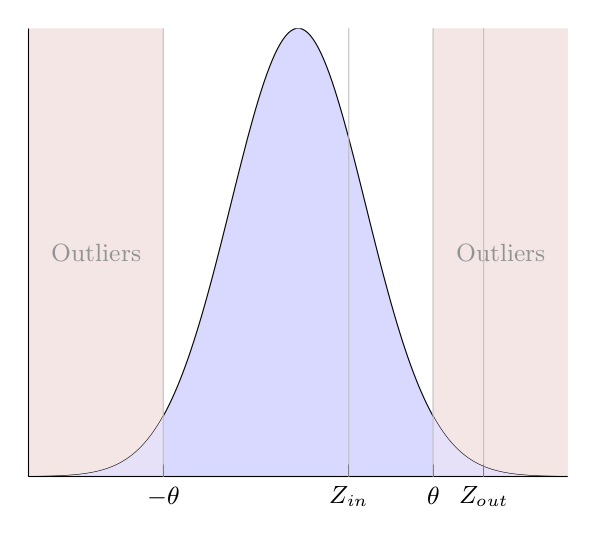
| Figure 1: Outliers. The histogram shows a normal distribution whose mean is at the peak. Red marks the values that are too far away from the mean. \(Z_{out}\) is a z-score that represents an outlier, whereas \(Z_{in}\) does not. |
Outliers are measurements that differ too much from expectation. Consider a sample of small measurements, say, temperature measurements from a frozen lake. This sample has a small expected value, represented by the sample mean, around the freezing point of water. A few large erroneous measurements, or even a single very large measurement such as the melting temperature of iron, can cause the mean to change significantly, thus misrepresenting the expected value. Outliers are therefore commonly removed from consideration to avoid damaging impact on processing.
Detecting outliers are done by calculating how much a measurement \(X_i\) differs from the average \(M_i\) of the sample measurements. The difference is normalized by dividing it with the standard deviation \(\sigma_i\). This is called the z-score:
$$\begin{eqnarray*} Z_i & = & \frac{X_i - M_i}{\sigma_i} \end{eqnarray*}$$
The simplest outlier detection uses a fixed threshold θ to determine whether or not a measurement is an outlier as illustrated in Figure 1. In mathematical terms, the outlier criterion is given by:
$$\begin{eqnarray*} |Z_i| & \ge & \theta \end{eqnarray*}$$
We use \(\theta\) to denote a threshold relative to the standard deviation \(\sigma\), and \(\Theta\) to denote an absolute threshold.
There are other ways to remove outliers, such as Pierce’s criterion that iterate over the data set applying stricter thresholds each iteration, but we are going to focus on those that are suitable for on-line processing. Let us look at a couple of those criteria.
h4. Three-sigma criterion
A commonly used threshold is three times the standard deviation. As the z-score already is divided by the standard deviation, the threshold becomes:
$$\begin{eqnarray*} \theta & = & 3 \end{eqnarray*}$$
With this threshold only the worst 0.3% of the measurements are marked as outliers.
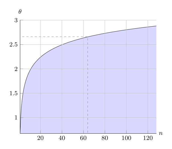 |
| Figure 2: Chauvenet’s criterion. Threshold θ becomes larger as the sample size grows. |
Another possibility is Chauvenet’s criterion defined as:
$$\begin{eqnarray*} \theta & = & \left| \Phi^{-1} \left( \frac{1}{4n} \right) \right| \end{eqnarray*}$$
where \(\Phi^{-1}(x)\) is the quantile function and \(n\) is the sample size.
The threshold depends on the sample size n as illustrated in Figure 2. For example, if we use a moving average algorithm with a window size of 64, then the threshold becomes \(\theta \approx 2.66\) as indicated with the dashed line.
Chauvenet’s criterion means that we accept greater deviations as the number of samples grows, and vice versa that we remove samples more aggressively for lower numbers of samples. We should be careful about sample sizes lower than 30, because that is the number of samples needed to approximate a normal distribution according to the central limit theorem.
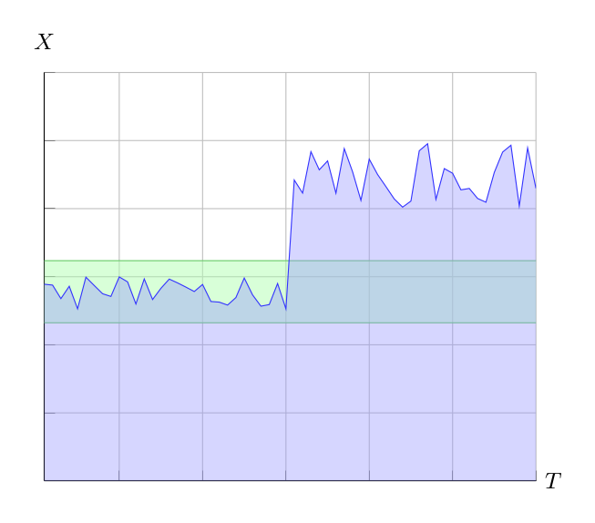 |
| Figure 3: Structural change. An abrupt change happens in the middle of the time-series. The first half of the samples, those inside the green area, are accepted, while the second half are all rejected as outliers. |
With this understanding of outliers, we can now proceed to the problem of structural change.
Figure 3 shows a time-series of measurements \(X_i\) received at time \(T_i\). Initially all samples are within the outlier threshold, those inside the green area, and are therefore accepted as valid measurements. Half ways through a structural change occurs and all subsequent samples are removed as outliers, those outside the green area. This is not what we would anticipate from a visual inspection of the graph: the second half of the samples ought to establish a new baseline with a new expected value, instead of being removed as outliers.
If measurements changes significantly due to a prolonged alternation of the sensory data, such as a photosensor when turning on the light, then there is a risk that this condition will go unnoticed because all new measurements are removed as outliers.
If we use outlier removal, then we also need a mechanism to detect structural changes.
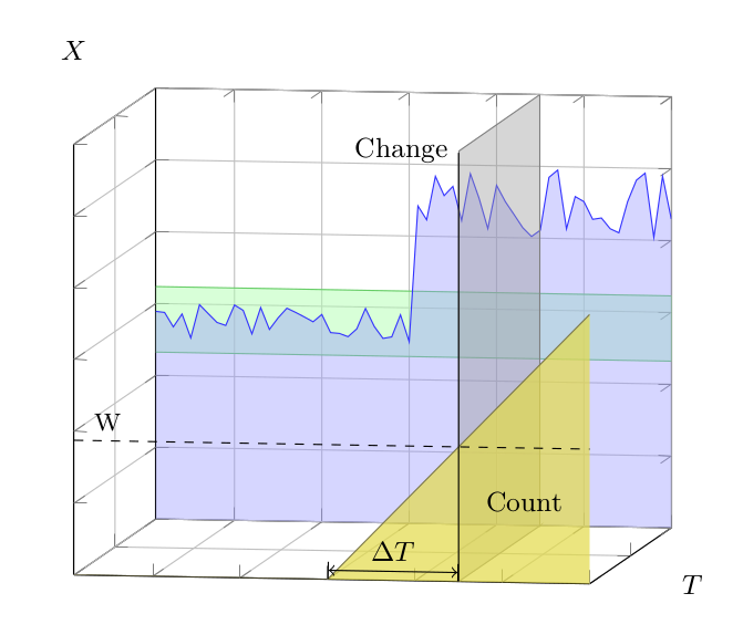 |
| Figure 4: Counters. The back plane is the same as Figure 3. The front plane shows an outlier count in yellow. Midways through, when the measurements becomes outliers, the count is incremented. A structural change is declared when the count reaches the watermark W. |
A simple approach to change detection is to count the number of consecutive measurements that are outliers. A structural change is declared when this count exceeds a counter watermark. Assuming that we receive measurements at a fixed pace, the reaction time before we declare a structural change is a fixed delay.
This counting approach can be extended in various ways. For example, we could differentiate between outliers above and below the green area respectively. Outliers above are counted up, and outliers below are counted down. A structural change is declared when the absolute value of the counter exceeds the watermark. Such an approach has the advantage of not confusing wild oscillations as structural change.
As another example we could have both high and low watermarks, and only declare a structural change when the counter exceeds the high watermark. Consecutive outliers that exceeds the low watermark, but not the high watermark, are used to adaptively modify the high watermark when we receive a measurement below the low watermark.
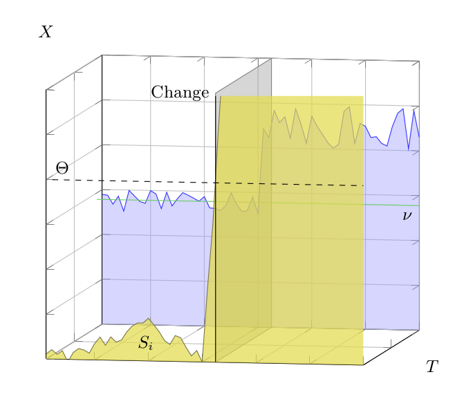 |
| Figure 5: CUSUM. The back plane shows the measurements \(X_i\) in blue, and the drift parameter \(\nu\) is marked by the green line. The front plane shows the accumulated deviation \(S_i\). A structural changes happens when \(S_i\) exceeds a threshold \(\Theta\). |
Another simple approach is to accumulate deviations over a number of consecutive measurements. When this accumulated value exceeds a threshold, a structural change is declared.
Whereas counters react on the amount of outliers, accumulated deviations react to the magnitude of the outliers. Therefore, the reaction time will depend on how large the deviations are: large structural changes are detected quickly, and small structural changes are detected more slowly.
For the cumulative sum a deviation is calculated as the difference between the current measurement \(X_i\) and an drift parameter \(\nu\).
$$\begin{eqnarray*} S_0 & = & 0 \\ S_i & = & \max(0, S[~i-1~] + X[~i~] - \nu ) \end{eqnarray*}$$
Notice that a positive difference, where \(X_i\) is greater than \(\nu\), increases the deviation, and negative difference reduces it. A structural change is declared when \(S_i\) exceeds the threshold \(\Theta\):
$$\begin{eqnarray*} S_i & \ge & \Theta \end{eqnarray*}$$
We could make cumulative sum more adaptive by changing the drift parameter ν from a constant into the expected value \(E_i\).
There are many more variations1 of this theme that we will not go into.
The previously mentioned approaches uses the number and magnitude of outliers, but not collected statistics of the measurements. For instance, the accumulation approach can mistake a single very large outlier as a structural change. We therefore continue with a change detection based on statistical concepts.
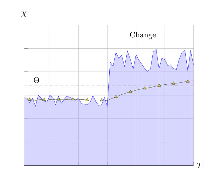 |
| Figure 6: Mean with threshold. The yellow line shows the running mean. A structural change is declared when the running mean exceeds the threshold \(\Theta\). |
A first approach is to declare a structural change when the sample mean \(M_i\) exceeds a threshold. For instance, we could use the exponential moving average to calculate \(M_i\) from measurement \(X_i\) in this way:
$$\begin{eqnarray*} M_1 & = & X_1 \\ M_i & = & \alpha X_i + (1 - \alpha)\, M_{i-1} \end{eqnarray*}$$
where \(\alpha\) is a smoothing factor.
The condition for structural change is then given by:
$$\begin{eqnarray*} M_i & \ge & \Theta \end{eqnarray*}$$
Be advised that the exponential moving average has a built-in bias towards the initial measurement \(X_1\). This bias can be removed by normalization.
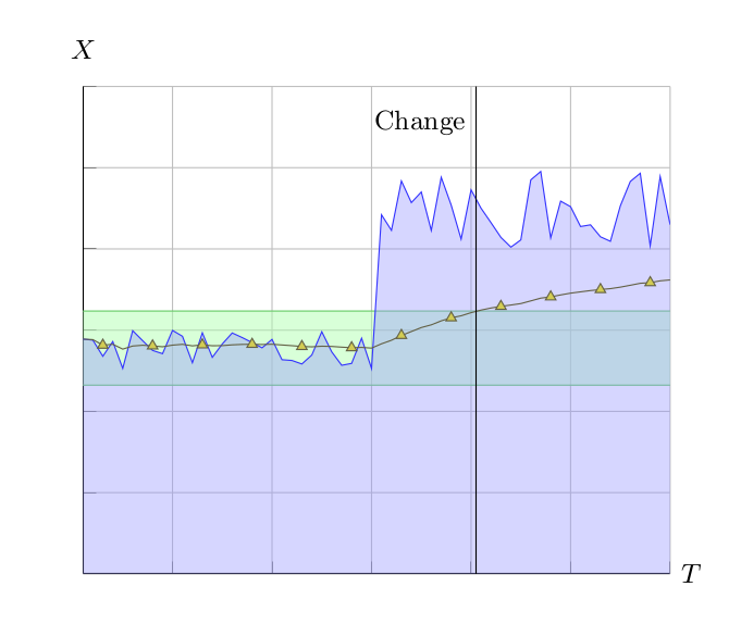 |
| Figure 7: Mean as outlier. The yellow line shows the running mean of the raw statistics. In the first half of the graph the raw mean is the same as the filtered running mean, but halfways through it grows to accommodate the outliers. A structural change is declared when the raw mean grows outside the green area. |
In a second approach we would like a more adaptable threshold \(\Theta\). We can incorporate the standard deviation to improve threshold. For that purpose we record two sets of statistics:
The basic idea of statistical change detection is quite simple: query if the mean of the raw measurements \(M_i\) has become an outlier according to the filtered statistics using the z-score:
$$\begin{eqnarray*} \frac{| M_i - M^\prime_i |}{\sigma^\prime_i} & \ge & \theta \end{eqnarray*}$$
The reaction time depends on the filters used. In the example shown in Figure 7, we used arithmetic mean of all measurements. If we want faster reaction times we could limit the statistics to the more recent measurements, for instance by using a moving average over a sliding window.
Fredrik Gustafsson, Adaptive Filtering and Change Detection, Wiley, 2000. ↩