| RSS | GitHub |
Calculating the mean of a sample can be done in various ways. A widely used method is the exponential moving average. We will show that this method has a bias towards the initial value, and present a way to remove the bias from the results.
|
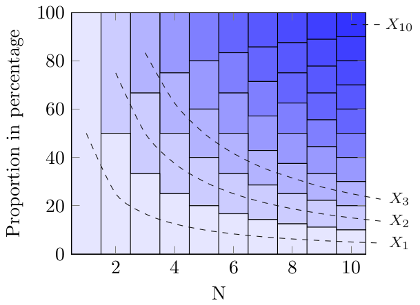
| Figure 1: Arithmetic Average. Each \(X_k\) value contributes in equal proportion as \(N\) is increased. |
We are going to start with the arithmetic mean to have a reference for the discussion below . The arithmetic mean of a sample \(\mathbf{X}\) is given by summing all values \(X_i\) in the sample and dividing the sum by the sample size \(N\):
$$\begin{eqnarray*} M & = & \frac{1}{N} \sum_{k=1}^{N} X_k \end{eqnarray*}$$
Let us visualize how this evolves as we add more values to the sample. When we add the first value \(X_1\) at iteration \(N = 1\) it will be equal to the mean. In other words, \(X_1\) will contribute 100% to the mean. When we add the next value \(X_2\) at iteration \(N = 2\), both \(X_1\) and \(X_2\) values will contribute 50% to the mean. This pattern will continue as we add even more values to the sample; no surprises here.
This is illustrated in Figure 1, where a stacked bar chart is used to show the proportion by which each value \(X_k\) contributes to the mean. The x-axis shows the development as more values are added to the sample.
Another technique for calculating the average is the exponential moving average given by recurrent formula:
$$\begin{eqnarray*} M_1 & = & X_1 \\ M_i & = & \alpha X_i + (1 - \alpha)\, M_{i - 1} \end{eqnarray*}$$
where α is a smoothing factor.
This technique has the clear advantage that we do not need to keep all previous values; we only need to store the previously calculated mean \(M_{i-1}\).
This leanness makes the exponential moving average quite popular in practical applications. For instance, it is used to calculate the smoothed round-trip time in the TCP protocol.
In the examples below we are going to use \(\alpha = \frac{1}{8}\), which happens to be the smoothing factor chosen by TCP. The general observations also hold for other values of \(\alpha\) albeit some thresholds may be different.
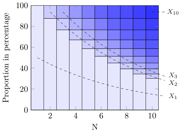 |
| Figure 2: Exponential Average. The initial value \(X_1\) contributes disproportionately. |
In order to better understand the recurrent formula above, we rewrite it as a sum:
$$\begin{eqnarray*} M^{\prime}_i & = & (1 - \alpha)^{i - 1} X_1 + \alpha \sum_{k = 2} (1 - \alpha)^{i - k} X_k \end{eqnarray*}$$
If we plot the evolvement of this formula just as we did for the arithmetic average, then we arrive at Figure 2. This graph shows a quite surprising feature of the exponential moving average, namely that the initial value \(X_1\) dominates the results for many iterations.
Normally we would expect that a value \(X_i\) contributes more to the result that then previous value \(X_{i-1}\). This is true for all values except the initial value \(X_1\).
We would furthermore expect that the most recently added value \(X_N\) contributes more that any of the other individual values \(X_i\), but that is not true for the first 16 iterations, where the initial value \(X_1\) continues to dominate.
The bad news is that the moving exponential average filter is critically dependent on a good measurement for the initial value. If the initial value is way off compared with the subsequent values, then it will take many iterations before this outlier is smoothed out.
The problem with the bias of the initial value is inherent in the recurrent formula for the exponential moving average:
$$\begin{eqnarray*} M_1 & = & X_1 \\ M_i & = & \alpha X_i + (1 - \alpha) M_{i - 1} \end{eqnarray*}$$
The first equation treats the initial value as a special value in order to get the subsequent values correct.
In the second equation, when we add a new value \(X_i\) it contributes only by a factor of \(\alpha\). For \(\alpha = \frac{1}{8}\) this becomes 12.5%. The remaining 87.5% comes from the previously calculated mean \(M_{i-1}\). This is generally a good solution, but we do have a bootstrap problem. This is solved by setting \(M_1\) to \(X_1\), but it also create the bias problem described in the previous section.
Let us dispense with the first equation in the recurrent formula as see if we can come up with a better solution.
In iteration 1 we calculate the contribution of the initial value \(X_1\) to be \(\alpha\) = 12.5%. In iteration 2 the second value \(X_2\) contributes 12.5% and \(X_1\) contributes \(\alpha \times (1 - \alpha)\) = 10.9%. We can derive the percentages for the remaining iterations from the second term in the non-recurrent formula \(M^{\prime}_i\).
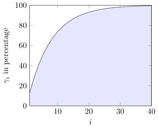 |
| Figure 3: Normalization factor. \(\gamma_i\) converges towards 100% as \(i\) grows. |
This gives us values that are much too small during the initial iterations, so we need to scale the 12.5% of \(X_1\) in iteration 1 to 100%, and the 12.5% + 10.9% for \(X_2\) and \(X_1\) in iteration 2 to 100%, and so on. In other words, in iteration 1 we must divide the calculated value by 12.5%, in iteration 2 by 12.5% + 10.9%, and so on.
We therefore introduce a normalization factor \(\gamma_i\). Let us write out some of the values to extrapolate a formula:
$$\begin{eqnarray*} \gamma_1 & = & \alpha & = & 12.5\% \\ \gamma_2 & = & \alpha + \alpha (1 - \alpha) & = & 12.5\% + 10.9\% \\ \gamma_3 & = & \alpha + \alpha (1 - \alpha) + \alpha (1 - \alpha)^2 & = & 12.5\% + 10.9\% + 9.6\% \\ \ldots \\ \gamma_i & = & \alpha \sum_{k = 1}^i (1 - \alpha)^{k - 1} \end{eqnarray*}$$
This formula can be rewritten as a recurrent formula:
$$\begin{eqnarray*} \Gamma_0 & = & 0 \\ \Gamma_i & = & \alpha + (1 + \alpha)\, \Gamma_{i - 1} \end{eqnarray*}$$
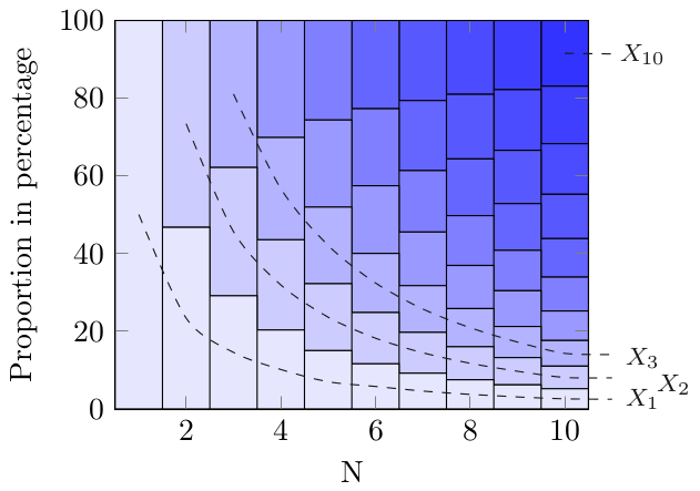 |
| Figure 4: Unbiased Exponential Average. |
We can incorporate this normalization factor into the exponential moving average and get an unbiased exponential moving average:
$$\begin{eqnarray*} MM_0 & = & 0 \\ MM_i & = & \alpha X_i + (1 - \alpha)\, MM_{i - 1} \\ M_i & = & \frac{MM_i}{\Gamma_i} \end{eqnarray*}$$
Figure 4 shows the results from the unbiased exponential moving average formula. It confirms that we get the expected results, namely firstly that normalization gives us correctly scaled values, and secondly that most recent values contributes more than older values.
Whereas the exponential moving average only maintains a single state variable \(M_i\), the unbiased version maintains two state variables \(MM_i\) and \(\Gamma_i\).