| RSS | GitHub |
Polynomials can be evaluated faster if we rewrite them and common wisdom tells us that a rewrite with fewer operations yields faster performance. For instance, Horner’s rule rewrites the polynomial to use the least number of multiplications. However, this does not yield the fastest performance on modern CPUs with instruction pipelining and vectorization.
An N-degree polynomial can be written as:
$$\begin{eqnarray*} f(x) & = & a_0 + a_1 x + a_2 x^2 + ... + a_N x^N \end{eqnarray*}$$
A naive implementation calculates the polynomial exactly as shown above. That is, \(x^n\) is calculated using \(n\) multiplications, \(x^{n-1}\) using \(n-1\) multiplications and so forth. Obviously that is inefficient, so let us improve on that using various rewriting schemes.
William George Horner, “XXI. A new method of solving numerical equations of all orders, by continuous approximation”, Philosophical Transactions of the Royal Society of London, 109, pp. 308-335, 1819. We can reduce the number of multiplications by applying Horner’s scheme where we pull out common \(x\) terms:
$$\begin{eqnarray*} f(x) & = & a_0 + a_1 x + a_2 x^2 +\ ...\ + a_n x^n \\ & = & a_0 + x\ (a_1 + a_2 x +\ ...\ + a_n x^{n-1}) \\ & = & a_0 + x\ (a_1 + x\ (a_2 +\ ...\ + x\ (a_{n-1} + a_n x) \ ... )) \end{eqnarray*}$$
This schema is a popular choice, and compilers often optimize the evaluation of polynomials using this rewrite.
Despite using the least amount of operations, this rewrite is not optimal for CPUs with instruction pipelining.
The CPU has to calculate the above expression inside-out. This means that each multiplication by \(x\) has to wait for the result of the adjacent parenthesis to become available. This is known as data dependency, and it causes the CPU pipeline to be stalled while waiting for the result.
Gerald Estrin, “Organization of Computer Systems: The Fixed Plus Variable Structure Computer”, IRI-AIEE_ACM Computer Conference, pp. 33-40, 1960. Another way to rewrite the polynomial is using Estrin’s Scheme where we pair the $I^{\text th}$ and $(I+1)^{\text th}$ monomials.
$$\begin{eqnarray*} f(x) & = & a_0 + a_1 x + a_2 x^2 +\ ...\ + a_n x^n \\ & = & (a_0 + a_1 x) + x^2\ (a_2 + a_3 x) + x^4\ (a_4 + a_5 x)\ +\ ... \end{eqnarray*}$$
All the parentheses are independent on each other, so we get fewer CPU pipeline stalls than with Horner’s scheme, which results in faster polynomial evaluation using Estrin’s scheme.
We still have to calculate \(x^{2j}\) for each group, but we can combine the groups using Horner’s scheme.
$$\begin{eqnarray*} f(x) & = & (a_0 + a_1 x) + x^2\ (a_2 + a_3 x) + x^4\ (a_4 + a_5 x)\ +\ ... \\ & = & (a_0 + a_1 x) + x^2\ ((a_2 + a_3 x) + x^2\ ((a_4 + a_5 x)\ +\ ...)) \\ \end{eqnarray*}$$
The above-mentioned rewrites does not leverage the built-in parallelism in modern CPUs in the form of vectorization.
William Dorn, “Generalizations of Horner’s rule for polynomial evaluation”, IBM Journal of Research and Development, 6(2), pp. 239-245, 1962. We can enable vectorization by using Dorn’s scheme, which rewrites the polynomial into \(k\) groups that can be computed independently. The result of these groups are then combined to produce the final result.
First we split the monomials into \(k\) polynomials called \(g_0(x)\) to \(g_{k-1}(x)\) that are independent on each other and therefore can be computed in parallel.
$$\begin{eqnarray*} g_0(x) & = & a_0 + a_k x^k + a_{2k} x^{2k} + ... \\ g_1(x) & = & a_1 + a_{k+1} x^k + a_{2k+1} x^{2k} + ... \\ & \vdots & \\ g_{k-1} & = & a_{k-1} + a_{k+k-1} x^k + a_{2k+1} x^{2k} + ... \\ \end{eqnarray*}$$
Then we combine these partial results.
$$\begin{eqnarray*} f(x) & = & g_0(x) + g_1(x)\ x + g_2(x)\ x^2 + ... +\ g_{k-1}(x)\ x^{k-1} \end{eqnarray*}$$
We can further optimize \(f(x)\) by using either Horner’s or Estrin’s scheme. For example, if we use Estrin’s scheme then we get.
$$\begin{eqnarray*} f(x) & = & \left(g_0(x) + g_1(x)\ x\right) + \left(g_2(x) + g_3(x)\ x\right)\ x^2 + ... \end{eqnarray*}$$
A good choice for \(k\) would be 4 or 8 because that is typically the number of floating point operations that can be computed in parallel. The exact number depends on your CPU though.
I have found no reference to this scheme in the literature. Estrin’s scheme can also be extended to better leverage the built-in parallelism. Rather than grouping two adjacent terms, we can group four adjacent terms, and then pull out common $x^{4j}$ where $j$ is the group number.
$$\begin{eqnarray*} f(x) & = & a_0 + a_1 x + a_2 x^2 +\ ...\ + a_n x^n \\ & = & (a_0 + a_1 x + a_2 x^2 + a_3 x^3) + x^4\ (a_4 + a_5 x + a_6 x^2 + a_7 x^3)\ +\ ... \end{eqnarray*}$$
This can also be combined with Horner’s scheme at the group level.
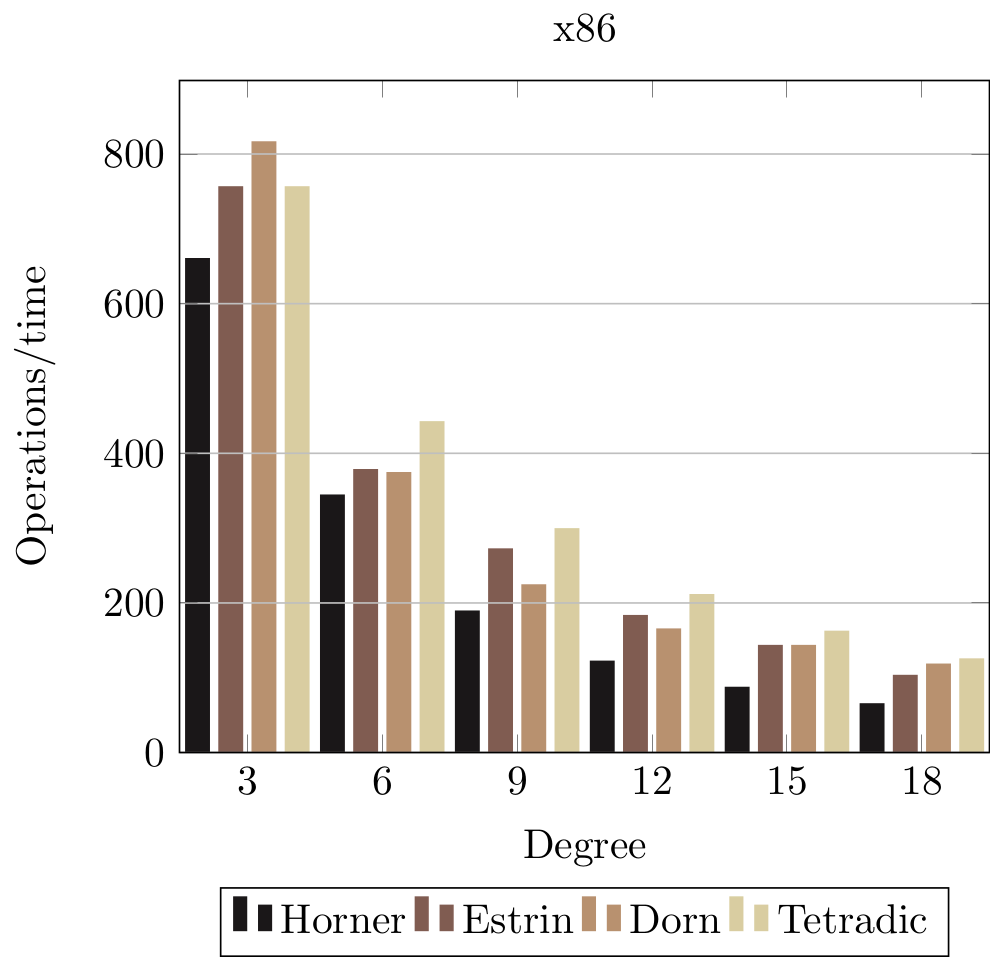
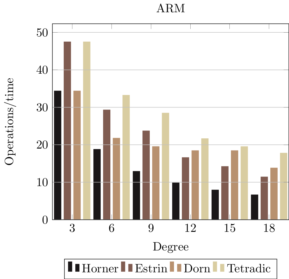
Let us see how these evaluation schemes compares to each other. We are interested in the relative performance, so do not put too much emphasis on the numerical values.
The horizontal axis shows polynomials of increasing size. The vertical axis shows performances measured by operations per time, so higher is faster.
The Dorn measurement are using a group size of 4.
|
|
The results show that Horner is consistently slower than the other rewriting schemes.
Pipeline stalls were measured using the Linux perf tool with uops_retired.total_cycles and uops_retired.stall_cycles. Horner’s scheme executes the fewest number of instructions but spends 40% of the time waiting on pipeline stalls. The Tetradic scheme executes 10% more instructions, but only spends 9% on pipeline stalls.
Notice that the relative performance gap grows along the horizontal axis. The Tetradic scheme is more than twice as fast as Horner at degree 18. Horner’s scheme only generates scalar instructions due to data dependencies, but the compiler is able to generate a certain amount of vectorized instructions for the other schemes, which accounts for the relative performance improvements.